Skip to content

The whole instrument,end to end.

The short version is on the front page. This is the long one: why dense seismic networks are priced out of reach, what averaging 32 motion sensors on one board actually buys, what sits on the two boards, how a reading travels from the ground to your browser, and how it compares with what already exists.

Seismology is priced like a luxury.

A geophone is an excellent instrument and a terrible way to build a network. Each one costs between $200 and $2,000, weighs enough to matter, breaks when it is dropped, and needs cable run to it before it is worth anything. Density, the thing that actually makes seismic data useful, is the first casualty.

A MEMS accelerometer costs about $3. It is the part in your phone. On its own it is far too noisy to do this job, which is why it has never seriously replaced the geophone.

VibeWatch does not build a better MEMS sensor. It buys 32 of them.

4.1×

Quieter, measured

$3

Per MEMS sensor

Cost per measurement point, USD
Traditional geophone$200 – $2,000+

Per sensor, before cabling

VibeWatch node≈ $250

Estimated, 32 sensors included

Averaging
in progress

01

Sensor averaged

1.0×

Quieter, in theory

True ground motion

Averaged output

One sensor

The problem is not sensitivity. It is noise.

A single $3 MEMS accelerometer hears the ground, but it also hears itself. Its own electrical and thermal noise sits on top of every reading, and there is no way to tell one from the other.

Two boards and a Raspberry Pi.

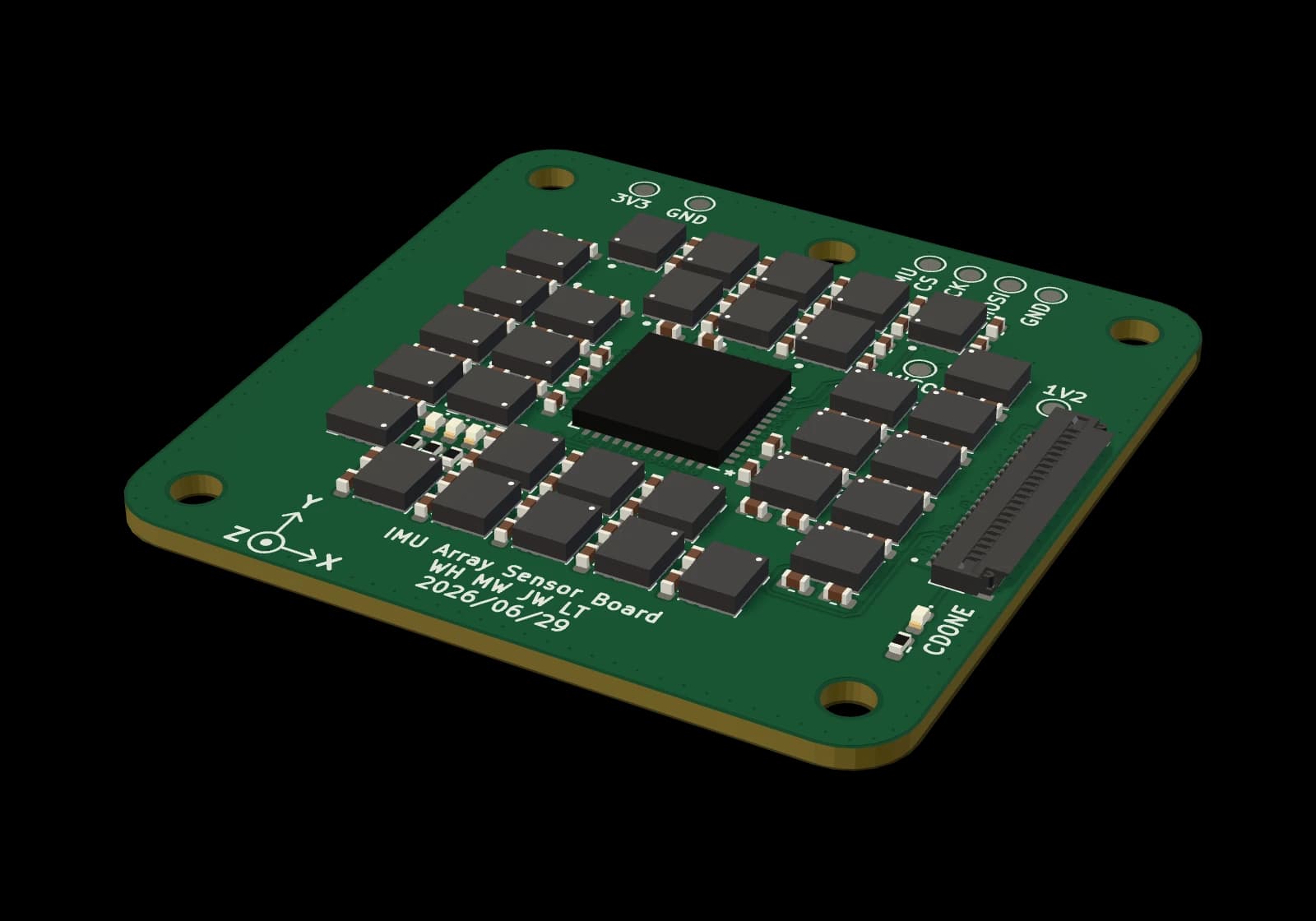
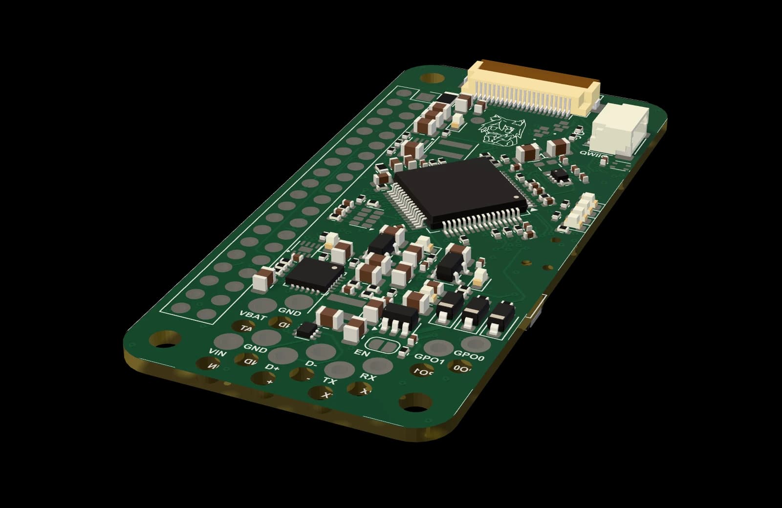
The sensor array fits in a square smaller than a coaster: 32 sensors around an FPGA that reads all of them at once. A flat cable takes the readings to the carrier board, which works with a Raspberry Pi to turn them into something you can plot.

The sensor board at an angle: 32 small black sensors in a grid around a square FPGA.The carrier board at an angle: a square microcontroller, power components and a flat-cable connector.
A

Sensor board

All 32 are read together and packed into a single transfer, so every sample in an average comes from the same moment.

Sensors
32 × ICM-42631, 6-axis
Aggregation
Lattice iCE40 FPGA, parallel SPI
Transfer
512 bytes per capture, one bus
Footprint
36 × 36 mm, six layers
Read
All 32 on a GPS-disciplined frame clock
Range
±2 g · ±15.625 °/s
B

Carrier board

The STM32 does everything that needs precise timing: steering its clock to GPS, reading the array, calibrating and averaging. The Pi does everything that needs a filesystem or a network. What leaves the node is already a result.

Real-time
STM32G474, 160 MHz with FPU
Host
Raspberry Pi 3A+, Wi-Fi and storage
Timing
u-blox MAX-M10N GPS, 40 MHz VCTCXO
Rate
50 to 2,000 averaged samples a second
Power
USB input and a battery
Sensing
SHT4x humidity, RV-3028 RTC

Sense, capture, process, stream.

01

Sense

32 ICM-42631 sensors feel the same ground motion. Each samples on its own internal clock, so the carrier reads all of them together on a frame clock steered by GPS, and every frame lands on the same timeline.

±2 g, GPS-timed frames

02

Capture

An iCE40 FPGA reads all 32 sensors in parallel and packs the readings into a single 512-byte SPI transfer. No sensor waits its turn, and the carrier board sees one tidy block instead of 32 conversations.

512 B per capture

03

Process

An STM32G474 on the carrier board corrects each sensor for its own manufacturing and mounting offsets, averages the corrected samples, and stamps the result with GPS time, up to 2,000 times a second. The work happens on the node, not in a data centre.

Per-sensor calibration · up to 2 kHz

04

Stream

A Raspberry Pi 3A+ connected to the carrier writes every frame to its storage. Within reach of Wi-Fi the node uploads as it records; out of range it keeps recording and uploads when a link returns. Sign in to see the map and play back recordings shared with you, including every public node.

Live or deployed · SD archive

Swipe to continue →

Everyone has one piece of this.

Dense networks exist. Cheap sensors exist. Good timing exists. Open data exists. What has not existed is one node that does all four at a price a city, a school or a research group can actually deploy.

Comparison of existing seismic monitoring systems by sensors per node, reach, and approach
SystemSensors / nodeReachIn short
UC Berkeley MAMA4 – 8Research prototypeProved MEMS averaging works for early warning, then stayed a research prototype.
Community Seismic Network1500+ nodesGenuinely dense across Los Angeles, but one sensor per node and no averaging.
Sercel QuietSeis · INOVA VectorSeisProprietaryCommercial surveyExcellent instruments, priced and aimed at oil and gas survey work.
Raspberry Shake1ConsumerAccessible and popular, with no multi-sensor averaging on the node.
China national MEMS network115,000+ stationsNational scale and real coverage, but still a single sensor at every station.
VibeWatchThis32Account · live or deployedCo-located averaging, GPS-disciplined timing, battery-backed on-node archive, community sharing for signed-in users, with public archive downloads planned.

Good seismology

Dense, well-timed ground motion data should not belong only to the institutions that can afford it. Create a free account to explore the network, or apply to host a node of your own.